(Last revised 2 January 2006.)
The examples shown here are for bivariate normal distributions in which both variables are scaled to have zero means and identical standard deviations. If the product-moment correlation is c, the probability density function is A exp(-(x2 + y2 - 2cxy)/2) for some constant A.
The general implication of the data presented below is that if one wants to make reliable predictions in individual cases of the value of one variable from another, the correlation coefficient serves primarily as an indication that no such predictions can be made. As the final table of this page shows, to be able to predict with 95% confidence which decile one variable lies in given the exact value of the other, a correlation of at least 0.997 is required. Even to predict only the sign of one variable from the other with 95% confidence requires a correlation above 0.995. Data which show that high a correlation are data that are so strongly correlated that no-one would bother to measure correlations in the first place.
One may have no concern with whether a prediction is correct in any particular case, but only with the overall success rate. In this case, a correlation of at least 0.5 is required to correctly predict just the sign of one variable from the other 2/3 of the time. Note that a 50% success rate is already guaranteed by chance.
The computations below have only been made for the bivariate normal distribution, but I believe they are unlikely to be substantially different for other bivariate distributions.
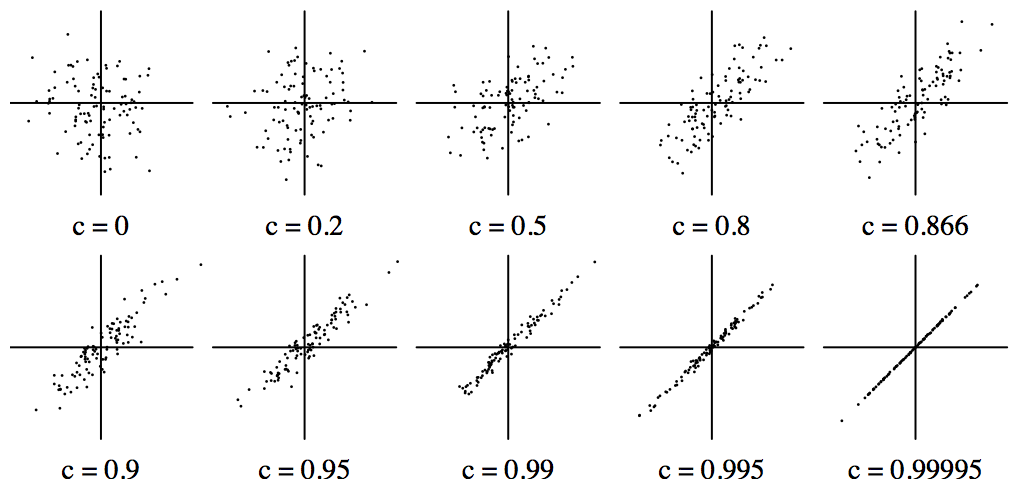
The figure shows scatter plots of 100 points for bivariate normal distributions of various correlations.
This figure shows contours of the density function of bivariate normal distributions for the same correlations as in the preceding figure. All of the contours of the bivariate normal distribution are concentric ellipses of the same shape, so only one need be plotted for each value of c.
The straight line is the regression line showing the most likely value of y given x. It is the straight line joining the two points on the ellipse where the tangent is vertical.

When the product-moment correlation is c, the covariance is c2. This is sometimes described as the amount of variance of y that is explained by or can be attributed to the variation of x. The remainder is the amount not so explained. (However, correlation is not causality: that which the above usage colloquially calls an explanation is not necessarily an explanation in the ordinary sense of the word.)
The improvement ratio is the ratio of the standard deviation of y given the value of x to the standard deviation of y when no information is given about x.
The mutual information of x and y is log2 of the improvement ratio. This is the amount of information in bits which one obtains about y from knowing the exact value of x.
All of these quantities are tabulated below.
| Correlation | Variance in y | Improvement ratio |
Mutual information (bits) |
|
|---|---|---|---|---|
| attributed to x | unaccounted for | |||
| 0 | 0 % | 100 % | 1 | 0 |
| 0.2 | 4 % | 96 % | 1.02 | 0.028 |
| 0.3 | 9 % | 91 % | 1.05 | 0.068 |
| 0.4 | 16 % | 84 % | 1.09 | 0.13 |
| 0.5 | 25 % | 75 % | 1.15 | 0.20 |
| 0.8 | 64 % | 36 % | 1.67 | 0.74 |
| 0.866 | 75 % | 25 % | 2 | 1 |
| 0.9 | 81 % | 19 % | 2.29 | 1.20 |
| 0.95 | 90.25 % | 9.75 % | 3.20 | 1.68 |
| 0.99 | 98 % | 2 % | 7.09 | 2.83 |
| 0.995 | 99 % | 1 % | 10 | 3.32 |
| 0.99995 | 99.99 % | 0.01 % | 100 | 6.64 |
To predict the sign of y, given x, the best that one can do is guess that y has the same sign as x. The first quantity tabulated below is the proportion of cases in which this guess is correct. A closed formula for this can be given: cos-1(-c)/π.
When x is close to zero, the guess will be little better than chance, but when x is large, the guess will be more reliable. Given the correlation coefficient, we can ask, how large must x be for the prediction of the sign of y to be correct most of the time? The last four columns of the table tabulate this for values of "most" equal to 95% and 99%. For each confidence value, the minimum absolute value of x in standard deviations is given, together with the probability that the absolute value of x is at least that large.
The extreme values in the first few rows of the table are primarily of theoretical interest: no real distribution can even be observed, let alone measured, at 11 standard deviations from the mean, and 4.3*10-28 % is equivalent to one water molecule out of 280 tons of water. *
[*: The only place where I can imagine there might be a counterexample to this is particle physics. One particle going zig when the other 2.3*1029 go zag might be within the bounds of detection.]
| Correlation | Probability of correct sign estimation |
Required rate of reliable classification | |||
|---|---|---|---|---|---|
| 95% | 99% | ||||
| min x | proportion of such x | min x | proportion of such x | ||
| 0 | 50 % | undefined | 0 % | undefined | 0 % |
| 0.2 | 56 % | 8.06 | 7.5*10-14 % | 11.40 | 4.3*10-28 % |
| 0.3 | 60 % | 5.23 | 1.71*10-5 % | 7.40 | 1.40*10-11 % |
| 0.4 | 63 % | 3.77 | 1.67*10-2 % | 5.33 | 9.91*10-6 % |
| 0.5 | 67 % | 2.85 | 0.4 % | 4.03 | 0.006 % |
| 0.8 | 80 % | 1.23 | 21.7 % | 1.74 | 8.1 % |
| 0.866 | 83.3 % | 0.95 | 34.2 % | 1.34 | 17.9 % |
| 0.9 | 85.6 % | 0.80 | 42.6 % | 1.13 | 26.0 % |
| 0.95 | 89.9 % | 0.54 | 58.9 % | 0.76 | 44.4 % |
| 0.99 | 95.5 % | 0.23 | 81.5 % | 0.33 | 74.0 % |
| 0.995 | 97.8 % | 0.17 | 86.9 % | 0.23 | 81.5 % |
| 0.99995 | 99.68 % | 0.016 | 98.7 % | 0.023 | 98.1 % |
We may wish to do more than merely predict the sign of y. The best prediction of the exact value of y from x is to guess that y is equal to cx. Given x, in what proportion of cases will this estimate of y differ from the correct value by an amount δ, where δ is such that only 10% of the whole population has a value of y within the range (x-δ ... x+δ)? This is tabulated here. (For the bivariate normal distribution, this happens to be independent of x.)
| Correlation | Prob. of estimation within ± half a decile |
|---|---|
| 0 | 10 % |
| 0.8 | 25 % |
| 0.9 | 36 % |
| 0.95 | 47 % |
| 0.99 | 78 % |
| 0.995 | 89 % |
| 0.997 | 95 % |
| 0.9985 | 99 % |
To be added to this page when I get round to it.